Authors Note: This is a follow-up post to my post about Playing With The Mandelbrot Set.
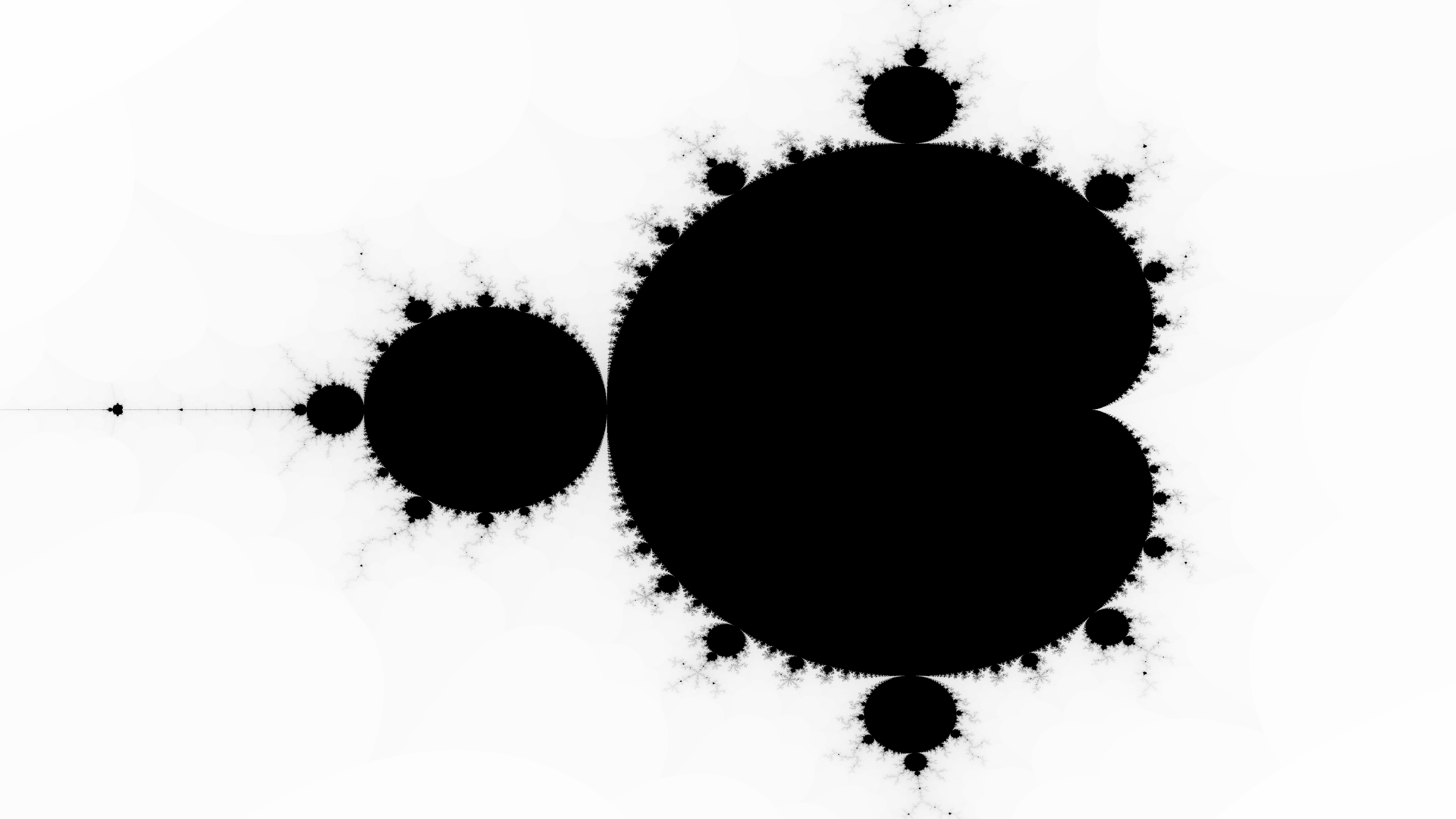
The Mandelbrot set is the set of all points on the complex plane where the function, f(n+1) = n^2 + c, continues to infinity without the result exceeding 2. It is the set of all complex numbers, n, applied to this function, where both the real and imaginary parts stay constrained.
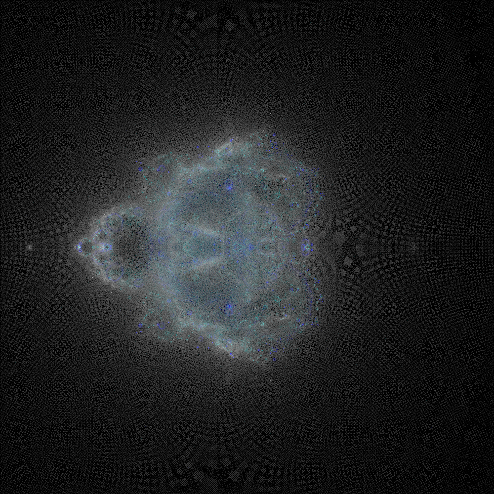
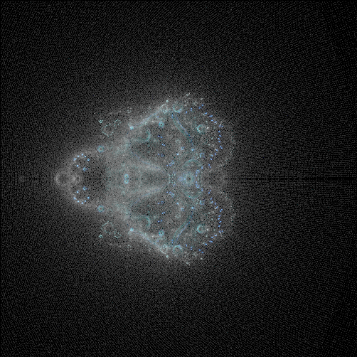
The Bhuddabrot is the inverse. It is the set of all numbers where the function outlined above does escape the bounds of 2. The image is a representation of the complex plane, where each iteration of every point is plotted in sequence.
In the Mandelbrot calculation, each pixel represents the number of iterations for that position. In the Bhuddabrot each pixel is a hit-counter describing the number of times a trajectory calculation has hit that point regardless of its starting position. The brighter Bhuddabrot pixel, the more times it was “hit” by a Mandelbrot trajectory.
The important distinction is, the Mandelbrot shows the contours of the shape, whereas the Bhuddabrot shows all the data points generated by completing the Mandelbrot calculation. They are simply different ways of displaying the same data.
Computation Challenges
The shape of the work is as follows: I needed to perform a Mandelbrot calculation many times. To be precise, I had to do this calculation three times for each pixel in the image. Why three times? Because to color the image, the calculation must be completed with slightly different parameters for each color: red, green, and blue.
The images along the way here are unclear. It’s a bit like looking into a pond. The colors red, green, and blue each represent a different depth in the pond. Red is “shallow” (least number of iterations), and blue is “deep” (most iterations), in the middle is green. As you transition from one color to the next, more details become apparent, but you can’t quite see the bottom.
Initially, I struggled with having some noise in the image. The problem was less apparent at lower resolutions, but at higher resolutions noise became increasingly problematic. I initially suspected the disturbance as being floating point errors. To resolve these issues, I needed to iterate on the code, meaning that I test the code, make changes to a new version, and repeat until I got something usable.
Unfortunately, a full-resolution render of the image took my laptop a smidge under 4-days. And that was before cranking the quality slider. Changing the code, then literally waiting for days to see what (if any) impact the change made would prevent the project from concluding anytime soon. Sounded like I needed a side-quest!
The good news is, each calculation point is independent of the others. In theory it would be possible to break the work into one “work unit” per “input-pixel” and then map the resulting heat-map onto an image.
Swoole
The next stop on my optimization journey was Swoole, a tool that allows users to write concurrent code. Using my previous render (let’s say 4 days) as a benchmark, and assuming I was able to divide the work evenly among CPU cores, a c8g.12xlarge AWS EC2 instance with 48 cores would require 2 hours. This napkin maths out to about $4 per run. If I forget to turn the machine off the $2/hr charge is going to get spendy quick.
Costs aside, I considered going slower on smaller instances. What would that look like?
Well, I would need a “work dispenser” that could yield work units from a generator. I also needed each “worker” to send its results back via some sort of channel. The last step was creating an image out of a reduction of all the results.
After a quick chat with Greg in the PHP Freelancer’s Guild Discord, we decided that because of the necessity of the shared data, Swoole wasn’t the best fit for the project. With Swoole, I must scale vertically and the type of work doesn’t fit well.
Note: If you have an idea for how to solve this problem with Swoole, leave a comment!
Queues And Workers
What if, instead of having a shared work dispenser, I broke the script into a few distinct steps? I thought this might work, and the steps I decided on are presented below:
- Pre-calculate the work to be done and insert each work unit into a queue.
- Workers pick up the work from the queue and write the resulting trajectory coordinates into a shared database.
- Finally, the database is queried for all coordinates in the image and some post-processing is done.
Let’s do some napkin math on what each simulation would cost.
- 6x
c8g.2xlargeinstances for two hours = $3.828 per run - 1x
db.t3.smallMariaDB instance = $36.32 per month
Ok, so the numbers don’t look great. One way or another the compute is going to cost about $4/run, but here I also have the added overhead of the database.
Another drawback is, there will be a network round-trip request for each work unit. Millions of work units are a lot of round-trip requests.
Trade Offs
With the Swoole method I was limited by the number of cores on any given physical machine. With the Queue route I was limited by the network overhead to distribute the work. Both methods cost about the same (minus the database).
The advantage of the queue worker method was that it was possible to scale elastically. In theory, I could set up an auto-scaling-group to hold a baseline (or even zero) number of workers, and set it to scale up to a bunch of workers to consume the workload.
If I went the queue route, I could adjust how quickly an image is generated by tuning the maximum number of instances it is allowed to spin up. Each image would still have the same overall price tag, but I would have a control for how quickly it would take to test changes to the code.
The Code
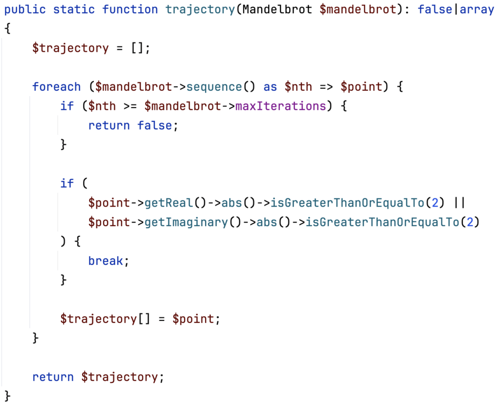
I was calculating a trajectory for a mandelbrot calculation which moves through a series of complex points. If I exceed my maximum number of iterations, I set it to return “false” as this point is inside the Mandelbrot set. Otherwise, the calculation would keep appending points within the bounds of the set to my trajectory until it found a point outside the set.
The code is below:
Noisy Image
The image generated still had noise in it. And it wasn’t as pretty as the images found on Wikipedia, for example. That simply would not do. The project was supposed to be print-quality and “noise” is not print quality.
Since I suspected the noise was coming from floating point errors, I spent some time employing my library (link here) rewriting everything to use my implementation instead. The gist of the change was that instead of working with approximately 14 decimal digits, I switched to working with 64 decimal digits and rounding off the remainder. I called the 64 decimal digit version “fancy math” and was certain that nothing bad would happen by employing it. I was wrong, but more on that later.
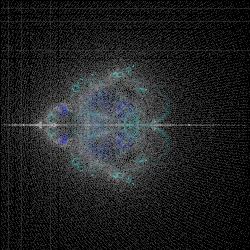
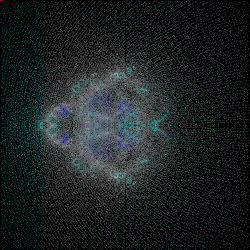
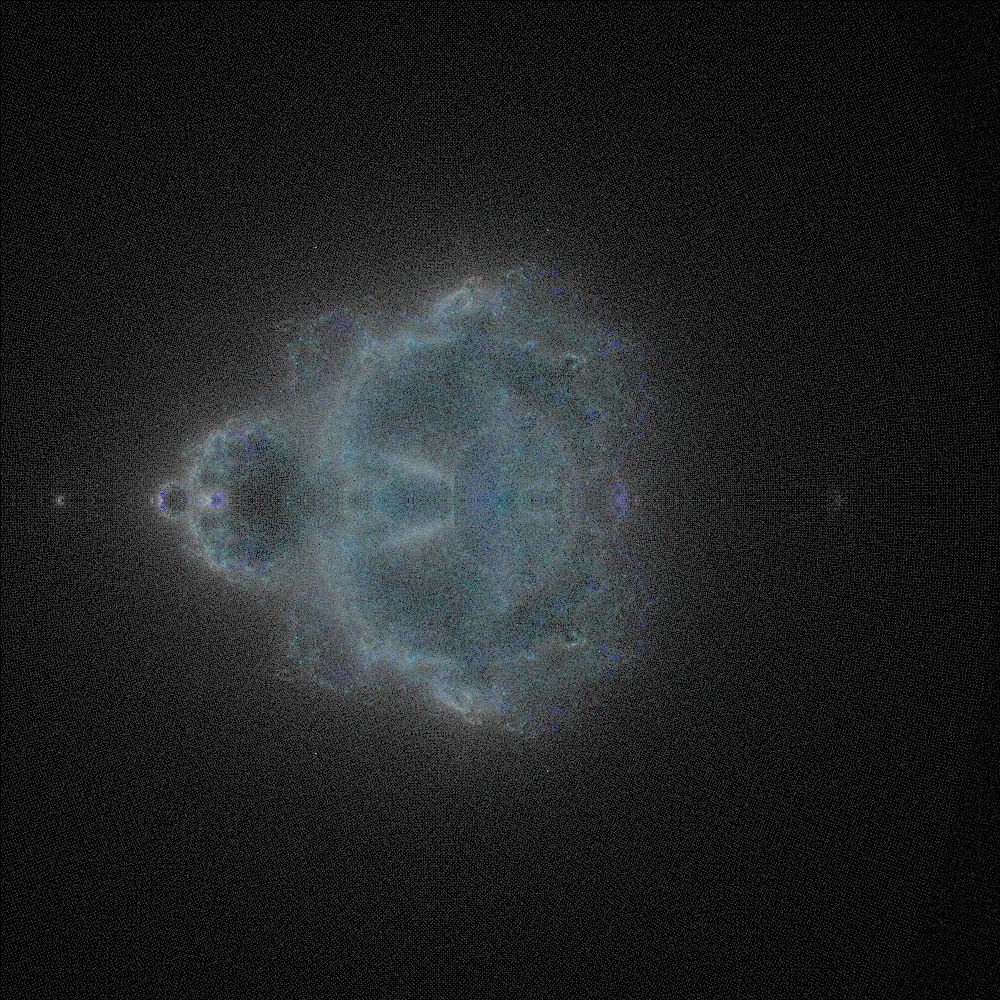
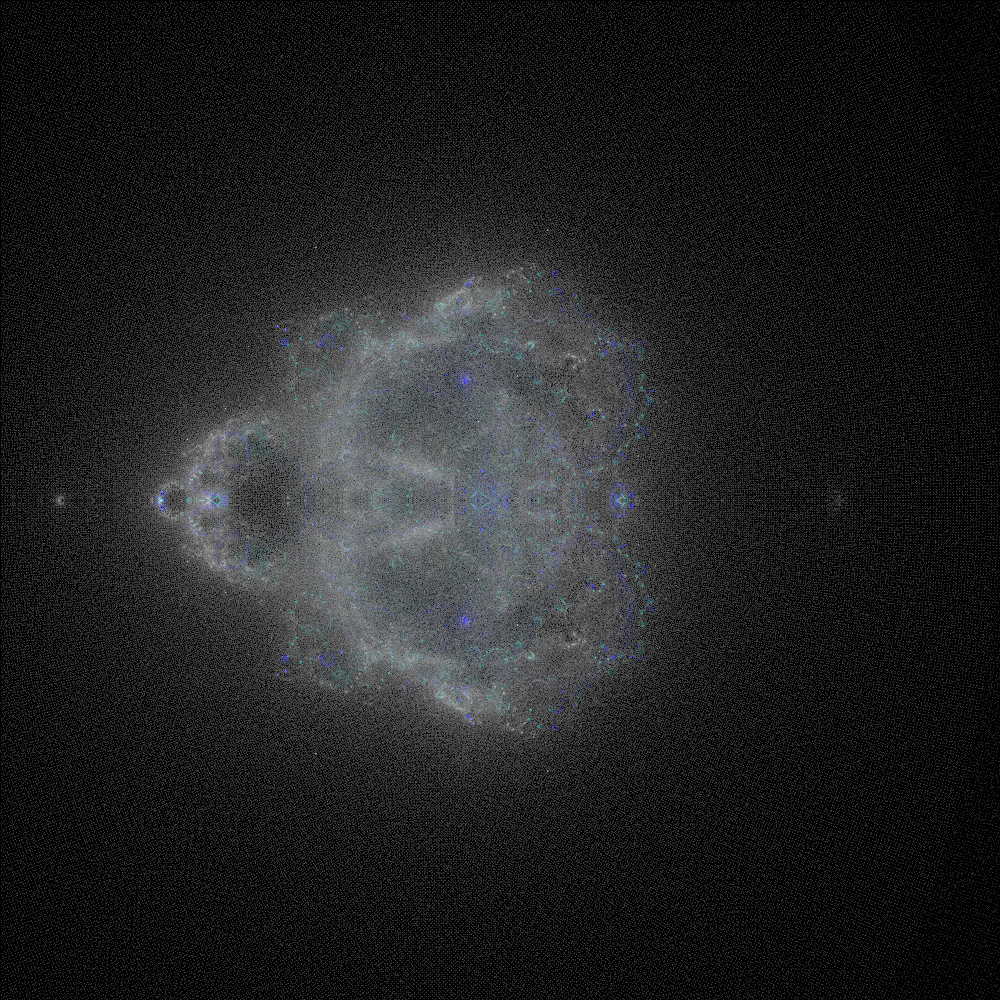
The initial results were promising. Here are side-by-side 250x250px renders of using the built-in math and the version using fancy math.
The Impossible Task
Here’s my line of thought: I needed to do arbitrary complexity calculations and get the really precise outline of a shape with an infinite curve.
The problem: You cannot have both.
The reason is simple. Calculating precisely is necessary to get a clear image. This blows up the memory usage. Suddenly the machine is n out of 5000+ iterations deep and out of RAM because it’s working with numbers of >=n*2 number of decimal places. It’s a technically solvable problem, but not in my lifetime.
At this point, I wondered, is this how Physicists feel about trying to capture an electron? They can either get the position or velocity, but not both.
I either had to tell a lie to get an image or accept the limitations of floating-point number capabilities. That, or use all the compute power in the universe to calculate the shape of an infinite curve. Truthfully, I’m not opposed to telling a small lie. I consoled myself by putting a disclaimer on the finished product.
Since I had to lie, I wanted to make it as small as possible, within reason. I’m not afraid of a small computer bill. It’s entertainment dollars. Whereas telling the whole truth would easily consume my whole paycheck.
The Final Code
I had to figure out how to do arbitrarily precise calculations on complex numbers. Naturally, someone else had already done the hard work with the brick/math library. Unfortunately, it doesn’t support complex numbers. Since complex numbers are just a logical extension of real numbers, I was able to extend brick/math to support complex numbers in another library I wrote.
The next step was removing all references to division. The division path rapidly consumes memory usage if not carefully contained. The answer is to use rationals.
“Oh boy, I’m smart”
Me, Judah Wright, 2025
The immediate next step was realizing that some numbers are going to be irrational by the nature of what we are trying to draw.
Suddenly, not feeling so smart.
Some massaging between rationals where appropriate and decimals where irrational got me over the hurdle.
“It’s only a small lie,” I told myself.
Elevating To The Cloud
I was not just throwing compute muscle behind a problem; I was being smart about it.
The Work Queue
Database Queue Driver
Right out of the box, I needed a database to store the intermediate results. For that, I used the Laravel database queue driver.
Unfortunately, the throughput of the job to queue the work is terrible. Terrible. Worse than local development on a sqlite database.
$ time php artisan app:queue-bhuddabrot-jobs 1000 1000
real    255m40.108s
Memory Store Queue Driver
A relational database is a bit overkill for the problem I was trying to solve. I was creating a big heap of work, then pulling the work off the queue as fast as we can. While this is doable with a relational database, I quickly hit a ceiling regarding how quickly the computer could pull items off the top of the pile.
Here’s the catch though, adding and subtracting work from the queue was not the slowest part of the operation. Running the actual calculations was the slowest part. So, while there was room for improvement, optimization efforts were chipping away at a relatively small slice of the total time spent.
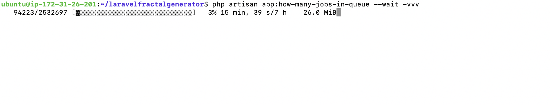
The final render has 243 million jobs to process. If each job is 1.5kb that adds up to 364.5GB just to hold the tasks. To ensure I wouldn’t blow the budget in cache storage space, I wrote some code to throttle the queue size. This meant the process was tied to how fast the work could be completed.
Infrastructure Benchmarks
I launched two servers, a c8g.medium (1-core) and a c8g.large (2-core) – each was configured to run with 4 workers. That meant that there were 8 workers total spread across 3 compute cores.
The “uppening” was upon us. If it worked, then all I’d have to do is create an auto scaling group of a proper size, worker number per core ratio, and maybe bump the database specs.
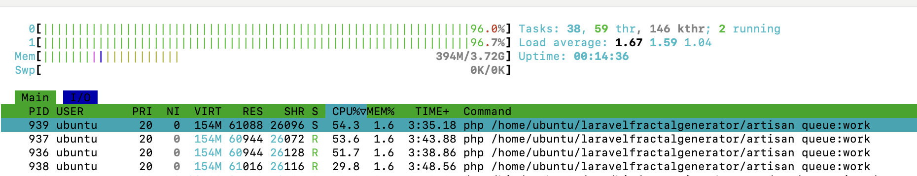
It ended up taking 10 hours to generate a 1,000px by 1,000px image that seemed acceptable. I was a move in the right direction.
Later, I ran a similar test, but tweaked the number of iterations for the red, green, and blue channels. I also set up an auto-scaling group to aim for 65% utilization on a maximum of 3 c8g.large spot-instance nodes, plus the c8g.medium “work dispensing” server. All 16 workers wrote to a t4g.small database back end. This test took around 7 hours from start to finish.
Scaling this up wasn’t a problem. I just need to tweak the auto-scaling group maximum node count to go faster. I even bought spot instances to avoid paying full price.
And then shit hit the fan.
I queued up the final render, and set the auto-scaling group to allow up to 20 spot instances. A week and $75 later, the progress bar says it’s at 10%. The easiest 10%. An estimated $750+ compute bill for a pretty picture was not in the budget.
According to the AWS billing dashboard, over the course of about 8 days I had sucked down 1368 computer hours. That’s 8 weeks of computer time. Surely, I’m using the wrong tool for the job.
I called my buddy Chris for help. We talked about how this task might be a great fit for GPU computing, whereas PHP runs on CPUs. If I were to put this into production, where I’d be generating many images instead of just one big one, I think GPUs would be better suited for the job. It’s silly to draw fractals in PHP.
Since PHP doesn’t run on GPUs, and doing arbitrary precision math on a different computing architecture sounds like a lot of learning, it seems this route is a dead end. This project was so close to being done! I didn’t want to start over from scratch.
Back To The Drawing Board
I stood back and beheld my creation. It had a work dispenser, a caching layer, work servers, and a database layer. What if, just like how lawn mower race drivers strip parts to go faster, I stripped parts off this monstrosity, just see how fast I could make it go.
Websockets
In the computer world, a “socket” is a special type of file. Scripts can both read from and write to a socket. They are unique in that they allow for inter-process communication, where one script can “talk to” another script. A “web socket” is the same process and idea, but instead of the special file being local, the special endpoint can be connected to over a network.
Websockets were the answer to how I was going to distribute the work. No database, no queue, just raw websockets.
The server
I slapped together some code to act as a “library” of sorts such that a worker could “check out” a unit of work. Then I put together a basic WebSocket server that would distribute work randomly from the library. Once a work unit has been “returned” with the trajectory for that point, the server updates the colors of the corresponding pixels in the resulting image.
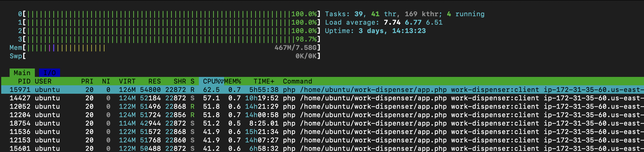
The client
Finally, a client script connects to the server, checks out work, and returns the necessary calculations. The returned coordinates could be quite a lot of data, so some buffering logic was necessary to send long results incrementally.
Further Optimizations
There were several optimizations along the way. The biggest optimization anyone can make is to simply “not do the work” in the first place. I thought more about the work being done. Each pixel input coordinate must have its calculation run three times with different iteration count limits. This is how you get the red, green, and blue channels.
Instead of doing the same work 3 times with different iteration counts, I completed the work once and counted the outputs. Then the channels were colored red, green, and blue depending on the iteration count. This optimization alone cut the work to render each image to a third. Being able to calculate all color channels from a single trajectory calculation was a big milestone.
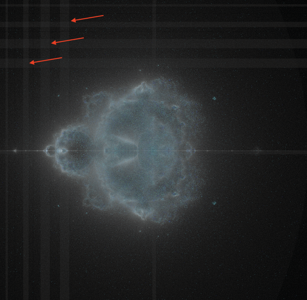
Problems With Base 10
Remember how I joked, “this rounding decision surely won’t haunt us later?” Well, now…
The new system was blazingly fast but the image noise came back. I hunted for, found, and eliminated all sorts of bugs in the math libraries. I was running simulations at 500x500px. Occasionally I’d run a 1000x1000px calculation. But render after render gave the same noise.
On happenstance, I wanted an intermediate quality image so I ran 768×768 and the noise was gone. There might be something there.
I consulted ChatGPT. It helped guide me to the answer.
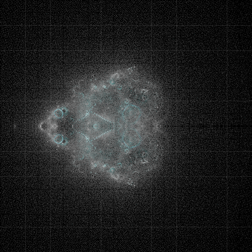
Turns out, that the overlaying grid is due to a small bias introduced with the combination of using a base-10 numbering system, and the necessity of rounding to the nearest base-10 decimal. This bias makes it subtly more likely that an escaping trajectory will land along a divisible-by-10 pixel space.
The solution was so simple!
The render cannot be of a size divisible by 10. Illustrated below is a 500px and a 502px wide image. Note that not only do the lines disappear, but it is a much sharper image.
The Final Render
Through the magic of “publishing when it’s done,” you didn’t have to wait for the week or so it took for the final render to render.
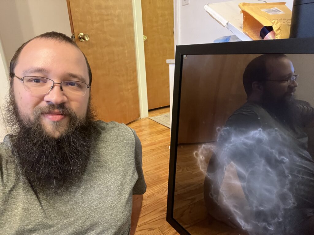
Anyways, enough stalling, here’s the final print, framed and ready to hang on the wall: